18.3 Simpson’s Rule

A way to interpret the trapezoidal method is that we approximate the integrand curve as a straight line, and then integrate that directly. The Simpson’s method does something similar, but instead of only using the integrand values at the boundaries it uses a third point (the midpoint) to approximate the integrand as a parabola.

The method approximates the integral as:

\[ \int_a^b f(x)~ dx \approx S(f) = \frac{b - a}{6} \left[ f(a) + 4 f\left(\frac{a + b}{2}\right) + f(b)\right] \]

with the derivation of this in the following section.

This can be shown [IntSimp1] to have an error of

\[ I(f) - S(f) = - \frac{1}{90} \left( \frac{b-a}{2} \right)^5 f^{(4)}(\xi) \]

for some \(\xi \in [a, b]\).

Derivation

Approximating \(f(x)\) as a Quadratic Polynomial

In order to approximate \(f(x)\) as a quadratic polynomial we can use a second order Lagrange polynomial. We construct this polynomial by using 3 data points \((a, f(a))\), \((m, f(m))\) and \((b, f(b))\).

\[ L(x) = f(a) \frac{(x - m)(x - b)}{(a - m)(a - b)} + f(m) \frac{(x - a)(x - b)}{(m - a)(m - b)} + f(b) \frac{(x - a)(x - m)}{(b - a)(b - m)} \]

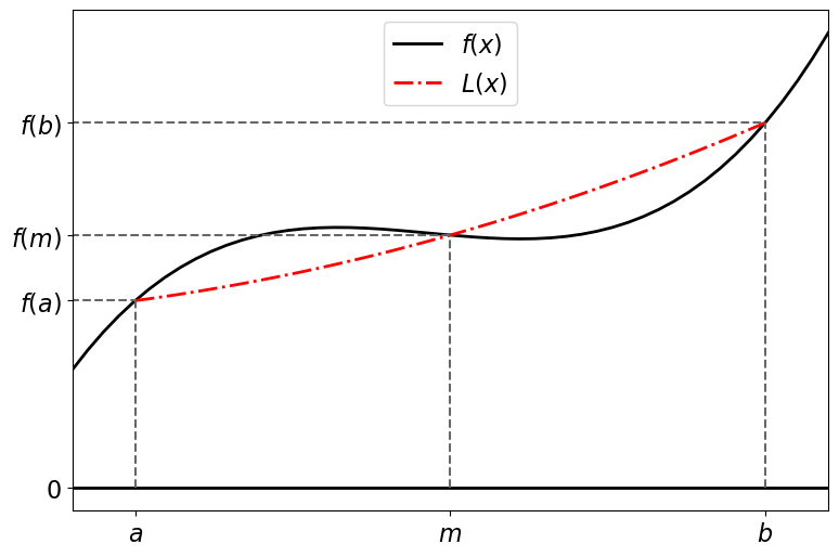
If we use the midpoint of \([a, b]\) for \(m\), i.e:

\[ m = \tfrac{1}{2} (a + b) \]

then we have

\[ m - a = b - m = \tfrac{1}{2} (b - a) \]

and the Lagrange polynomial becomes:

\[ L(x) = \frac{2}{(b - a)^2} \big[ f(a) (x - m) (x - b) - 2 f(m) (x - a) (x - b) + f(b)(x - a)(x - m) \big] \]

Integrating \(L(x)\)

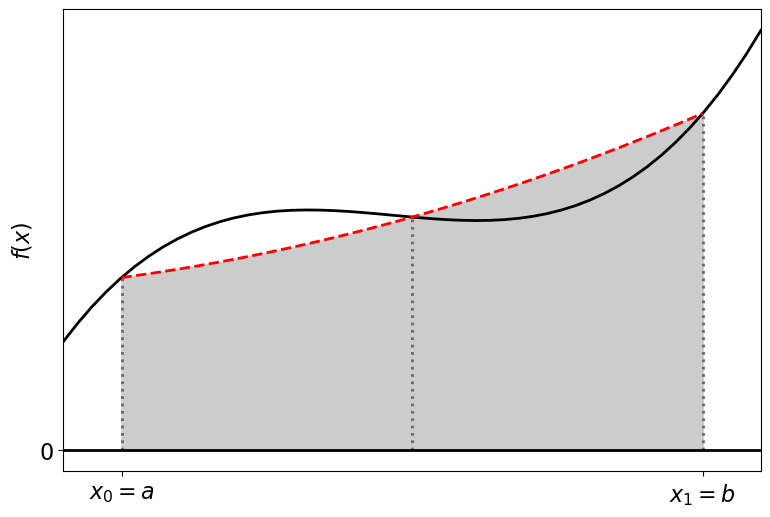
Now, we wish to approximate the integral of \(f(x)\) as the integral of our Lagrange polynomial:

\[ \int_a^b f(x)~ dx \approx \int_a^b L(x)~ dx \]

illustrated in the figure below:

by substituting the variable:

\[ u = \frac{x - m}{b - m} = 2 \frac{x - \tfrac{1}{2} (a + b)}{b - a} \]

into the integral of \(L(x)\) we find that:

\[ \int_a^b L(x)~dx = \frac{b - a}{6} \left[ f(a) + 4 f\left(\frac{a + b}{2}\right) + f(b) \right] \]

thus, we approximate the integral of \(f(x)\) as:

\[ \int_a^b f(x) ~dx \approx \frac{b -a}{6} \left[f(a) + 4 f\left(\frac{a + b}{2}\right) + f(b) \right] \]

Alternative Derivation

Another way to see the Simpson’s rule is as a weighted average of the midpoint and trapezoidal rules:

2/3 midpoint + 1/3 trapezoidal

Mathematically:

\[\begin{align*} \int_a^b f(x)~ dx &\approx \frac{2}{3} f\left(\frac{a + b}{2}\right) (b - a) + \frac{1}{3} \times \frac{1}{2} (b - a) [f(a) + f(b)]\\ &\approx \frac{b - a}{6} \left[ f(a) + 4 f\left(\frac{a + b}{2}\right) + f(b)\right]\\ \end{align*}\]

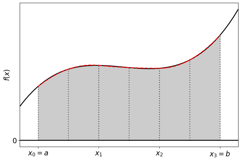
Composite Simpson’s Rule

As before we can improve the accuracy of our solution by subdividing the interval and calculating the integral using Simpson’s rule for each subinterval.

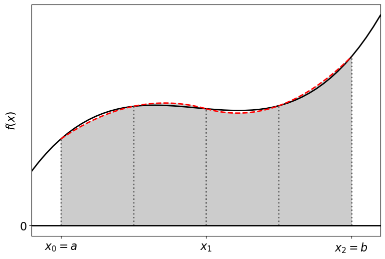
The composite Simpson’s rule is given by:

\[\begin{split} \int_a^b f(x)~ dx \approx S_n (f) = \sum_{i = 0}^{n-1} \frac{x_{i+1} - x_i}{6} \left[ f(x_i) + 4 f\left(\frac{x_{i} + x_{i+1}}{2}\right) + f(x_{i+1})\right]\\ \end{split}\]

If we use equal sized sub-intervals, then we have that:

\[ x_i - x_{i -1} = \frac{b - a}{n} \equiv h \]

taking this into account and the values of \(f(x_i)\) which are repeated in the sum, the composite Simpson’s rule can be simplified to:

(21)\[ S_n(f) = \frac{h}{6} \left[ f(a) + 2 \left\{\sum_{i = 1}^{n-1} f(a + ih)\right\} + 4 \left\{\sum_{i =0}^{n-1} f\left( a + \left(i + \tfrac{1}{2}\right) h \right)\right\} + f(b) \right] \]

The (global) error for this can be determined [IntSimp1] as:

(22)\[ I(f) - S_n (f) = - \frac{b - a}{180} h^4 f^{(4)}(\xi) = O(h^4) \]

for some different \(\xi \in [a, b]\).

Composite Simpson’s Rule with a Discrete Data Set

We can use the Simpson’s rule to integrate a discrete set of data, though there are some requirements that the data set must fulfill in order to do so.

Again, consider the data set \((x_i, y_i)\) for \(i = 0, \dots, n\), where

\[ f(x_i) = y_i \]

Approximating the integral of the data using Simpson’s rule is a lot less straight forward than the Trapezoidal rule as we can’t calculate \(f\left((x_{i -1} + x_i)/2\right)\) directly.

If the \(x_i\) values are uniformly spaced (with \(x_i - x_{i-1} = \Delta x\)) and there is an odd number of data points, we can pair up the intervals between the points. Treating each pair of subintervals as a single subinterval, we can use the middle \(x\) values as the midpoints. In other words, for even \(i= 2j\), the \(x_{2j}\) are used as the boundaries of the sub-intervals; for odd \(i = 2k -1\), the \(x_{2k-1}\) are used as the midpoints of the subinterval. Thus the integral is approximated as:

\[ \int_{x_0}^{x_n} f(x)~dx \approx \frac{\Delta x}{3} \left[y_0 + 2 \left\{\sum_{i = 1}^{n/2 - 1} y_{2i}\right\} + 4 \left\{\sum_{i=1}^{n/2} y_{2i-1}\right\} + y_n \right] \]

Note that

\[ \frac{b - a}{6 n} = \frac{2 \Delta x}{6} = \frac{\Delta x}{3} \]

as each subinterval is made up of two intervals of length \(\Delta x\) each.

References

[IntSimp1] (1,2)

James F. Epperson. An Introduction to Numerical Methods and Analysis. John Wiley & Sons, Inc., Hoboken, New Jersey, second edition edition, 2013.