1 Applying Richardson Extrapolation to Euler’s Method

As Euler’s method is derived using Taylor expansions, they have the appropriate properties to apply Richardson’s extrapolation.

Note

Remember For a numerical method of the form:

\[ A = A_0(h) + a_0 h^{k_0} + a_1 h^{k_1} + ... \]

with \(0 < h < 1\) and \(k_0 < k_1 < k_2 < ...\). Richardson extrapolation can be appied recursively to imprive the approximation:

\[ A_{i+1} (h) = \frac{t^{k_i} A_i \left( \tfrac{h}{t} \right) - A_i(h)}{t^{k_i} - 1} \]

with leading error of \(O(h^{k_{i + 1}})\). Error can be estimated as:

\[ E_{i+1}(h) = A_{i+1}(h) - A_i \left( \tfrac{h}{t} \right) \]

Let’s apply a single iteration of Richardson’s extrapolation to Euler’s method. Remember that Euler’s method is defined as:

\[ y_{i+1} = y_i + h f(x_i, y_i) + O(h^2) \]

In the notation used for Richardson extrapolation:

\[ A_0 (h) = y_i + h f(x_i, y_i) \]

and \(k_0 = 2\), \(k_1 = 3\), etc.

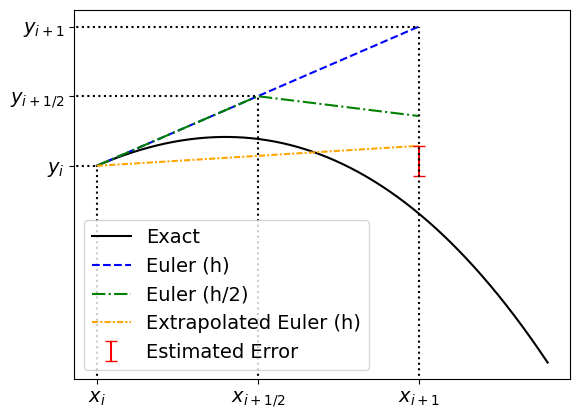
Now we need to make a choice for \(t\) to determine \(A_0 (h/2)\), a common choice is \(t = 2\). To determine \(A_0 (h/2)\) at \(x_i + h\), we will take 2 Euler steps with step-size \(h/2\):

\[\begin{align*} y_{i + 1/2} &= y_i + \tfrac{h}{2} f(x_i, y_i)\\ &\\ A_0 \left( \tfrac{h}{2} \right) &= y_{i + 1/2} + \tfrac{h}{2} f\left(x_i + \tfrac{h}{2}, y_{i+1/2} \right) \end{align*}\]

from which we can calculate the first iteration of the Richardson extrapolation:

\[ A_1(h) = \frac{4 A_0 \left( \tfrac{h}{2} \right) - A_0 (h)}{3} \]

with estimated error:

\[ E_1 (h) = A_1 (h) - A_0 \left( \tfrac{h}{2} \right) \]

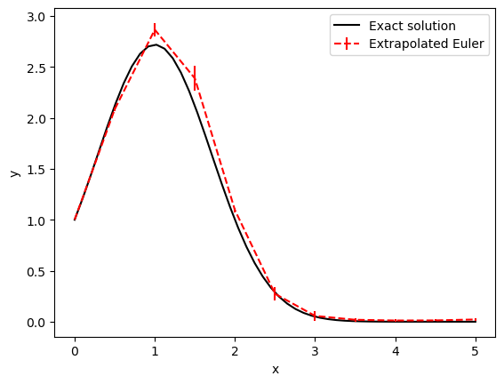
Worked Example

Consider the ODE:

\[ \frac{d y}{dx} = - 2 (x - 1) y \]

which has the exact solution:

\[ y(x) = e^{- (x - 1)^2 + 1} \]

Let’s solve this ODE from \(x = 0\) to \(1\) with a step-size of \(0.5\) using a single iteration of Richardson extrapolation applied to Euler’s method and compare this to the exact solution.

import numpy as np
import matplotlib.pyplot as plt

x0, y0 = 0, 1
h = 0.5
x_end = 5

#The ODE function
def f(x,y):
    return -2 * (x - 1) * y

def y_exact(x):
    return np.exp( -(x - 1)**2 + 1 )


x_extrap = np.arange(x0, x_end + h, h)
y_extrap = np.zeros(x_extrap.size)
y_extrap[0] = y0
e_extrap = np.zeros(x_extrap.size)
#Note there is no error estimate for (x0, y0)
e_extrap[0] = 0

for i, x in enumerate(x_extrap[:-1]):
    #Euler step
    y_h =  y_extrap[i] + h * f(x, y_extrap[i])

    #Half-euler step
    y_h2 = y_extrap[i] + 0.5 * h * f(x, y_extrap[i])
    y_h2 = y_h2 + 0.5 * h * f(x + 0.5 * h, y_h2)

    #Extrapolation
    y_extrap[i+1] = (4 * y_h2 - y_h) / 3
    e_extrap[i+1] = y_extrap[i+1] - y_h2

#Plotting the solution
x_plot = np.linspace(x0, x_end)
fig, ax = plt.subplots()

ax.plot(x_plot, y_exact(x_plot), 'k-', label = 'Exact solution')
ax.errorbar(x_extrap, y_extrap, yerr=np.abs(e_extrap), 
            ls='--', color='red', label='Extrapolated Euler')
ax.set_xlabel('x')
ax.set_ylabel('y')

ax.legend()

plt.show()