18.1 Midpoint Rule

In the midpoint rule you approximate the area under the curve as a rectangle with the height as the function value at the midpoint of the interval:

\[ \int_a^b f(x)~ dx \approx M(f) = f\left(\frac{a + b}{2}\right) (b - a) \]

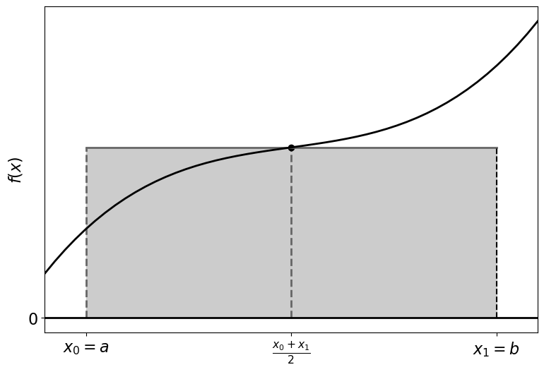
Which can also be derived from a Taylor expansion [IntMid1].

This can be shown to have an error of:

\[ I(f) - M(f) = \frac{1}{24} (b - a)^3f''(\xi) \]

for some \(\xi \in [a, b]\). Although we can’t actually determine the relevant \(\xi\), we can find an upper bound for the error by finding the maximum of \(f''\) in the interval of \([a, b]\). Note as the error is proportional to \((b - a)^3\), for a large interval (larger than 1) the midpoint rule is not very accurate.

Composite Midpoint Rule

For a more accurate solution we can subdivide the interval into small sub-intervals, approximate the integral values for the sub-intervals and sum these. Let’s illustrate this for the midpoint rule:

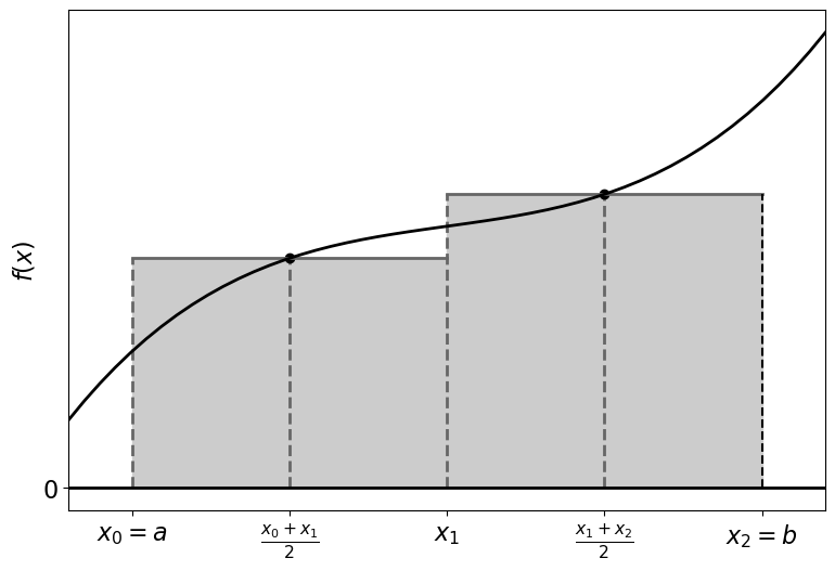
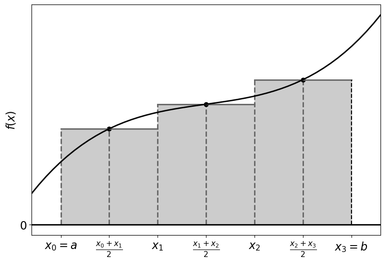
For \(n\) subdivisions:

\[ \int_a^b f(x)~ dx \approx M_n(f) = \sum_{i=0}^{n-1} (x_{i+1} - x_{i}) f\left(\frac{x_{i+1} + x_{i}}{2}\right) \]

If these divisions are equal, then

\[ x_{i+1} - x_{i} = \frac{b - a}{n} \equiv h \]

which gives us:

(17)\[ M_n(f) = h \sum_{i=0}^{n-1} f\left(a + \left(i + \tfrac{1}{2}\right) h \right) \]

This can be shown [IntMid1] to have an (global) error of:

(18)\[ I(f) - M_n(f) = \frac{b - a}{24} h^2 f''(\xi) = O(h^2) \]

for some different \(\xi \in [a, b]\). Remember, that we want to choose \(n\) so that \(h < 1\) to reduce the error.

References

[IntMid1] (1,2)

James F. Epperson. An Introduction to Numerical Methods and Analysis. John Wiley & Sons, Inc., Hoboken, New Jersey, second edition edition, 2013.