Simple Plots with Pyplot
The Pyplot module of Matplotlib acts as an interface to the Matplotlib package. This gives us access to a library of 2-dimensional plotting functions. The standard way of importing Pyplot is:
import matplotlib.pyplot as plt
As a first example, let’s plot the line \(y = x^2\):
import numpy as np
import matplotlib.pyplot as plt

x = np.linspace(0, 2, 100)
y = x*x

plt.plot(x, y) #Plots a line

plt.xlabel('x') #x-axis label
plt.ylabel('y')

plt.show() #Visualizes the plot
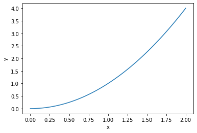
where:
plt.plot()plots a straight line, which is one of the many types of plots available in the module (see the Thumbnail Gallery for more).The
plt.xlabel()andplt.ylabel()functions set the labels for the x and y-axis of the plot to the given arguments respectively.plt.show()shows the current figure (discussed in the following section). In the regular Python environment this function will pause the code and bring up a window containing the plot. Elements of the plot can be edited in this window and this plot can be saved. Closing the window resumes the script.In Jupyter Notebook, running
plt.show()will display the plot in the cell output and will not pause the script.
Figures
A Matplotlib figure contains plot elements, for example a set of (or multiple sets of) axis, a title etc. Figures can be created using
fig = plt.figure()
When using plt.plot() Matplotlib will automatically add the plot to the last figure that was defined. Refer to the page Scientific Packages/Matplotlib/Subplots page for accessing the figure axis directly.
If you want to specify the dimensions of the plot, you can create a figure with the first positional or keyword argument:
fig = plt.figure(figsize = (width, height) )
where figsize (a 2-tuple of width and height) is in inches.
For more information on the figure class see the documentation.
Saving Figures
You can save figures using the
plt.savefig(filename)
function, where filename is the filename of the image to be saved. If a file extension is specified, the image will be saved using that type, the default type is a PNG.
This will save the current figure, if you want to save a particular figure then you can use fig.savefig().
If you’re not specifying the figure, make sure to save before you call plt.show() as this will clear the figure.
Line Color
You can specify the line color for the plot using either a positional (single letter) argument:
plt.plot(x, y, 'r')
or using a keyword argument:
plt.plot(x, y, color = 'red')
where the examples above both produce red lines, for example:
x = np.linspace(0, 2, 100)
y = x*x

plt.plot(x, y, 'r')

plt.xlabel('x')
plt.ylabel('y')

plt.show()
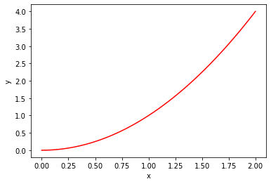
The list of colors, as found in the Matplotlib documentation, is:
Single Letter |
Full Name |
|---|---|
b |
blue |
g |
green |
r |
red |
c |
cyan |
m |
magenta |
y |
yellow |
k |
black |
w |
white |
Shades of gray can be given as a string representation of a float between 0 and 1, for example:
color = '0.75'
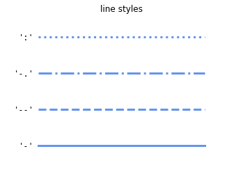
Line Style
Similar to the color of the plot, you can also set the line style, either as a positional argument:
or as a keyword argument:
Note that both the color and line style can be combined when set using the positional argument.
The reference for the lines given below is taken from the documentation:
Marker
In addition to line style and color, you can specify a marker. The markers are placed at each data point. The possible markers are listed in the documentation, as an example let’s plot the data points as circles ('o' in the positional argument, or marker = 'o' as a keyword argument):
x = np.linspace(0, 2, 10)
y = x*x

plt.plot(x, y, 'ro')

plt.xlabel('x')
plt.ylabel('y')

plt.show()
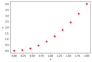
As you can see the line style is set to 'None' by default if a marker is specified without a line style.
Legends
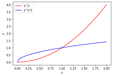
You can add a legend to your figure by labeling the plots with the keyword argument label and calling the plt.legend() function:
x = np.linspace(0, 2, 100)

plt.plot(x, x*x, 'r', label = 'x^2')

plt.plot(x, np.sqrt(x), 'b', label = 'x^0.5')

plt.xlabel('x')
plt.ylabel('y')

plt.legend()

plt.show()
