.ipynb .pdf

repository open issue

Binder

Contents

Midpoint Rule

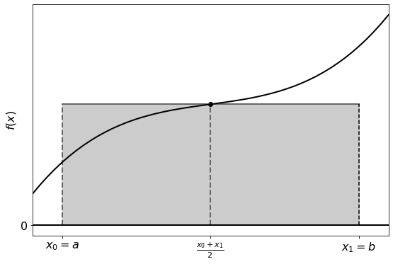
In the midpoint rule you approximate the area under the curve as a rectangle with the height as the function value at the midpoint of the interval:

\[ \int_a^b f(x)~ dx \approx f\left(\frac{a + b}{2}\right) (b - a) \]

Composite Midpoint Rule

For a more accurate solution we can subdivide the interval further, constructing rectangles for each subinterval, with the function value of the midpoint used as the height:

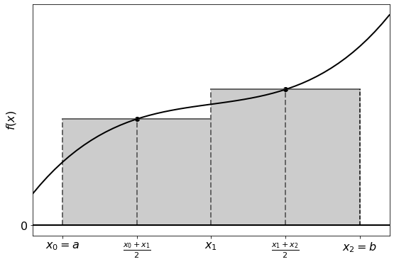
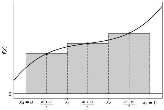
For \(n\) subdivisions:

\[ \int_a^b f(x)~ dx \approx \sum_{i=1}^n (x_i - x_{i-1}) f\left(\frac{x_i + x_{i-1}}{2}\right) \]

If these divisions are equal, then

\[ x_i - x_{i-1} = \frac{b - a}{n} \]

which makes the approximation:

\[ \int_a^b f(x) ~dx \approx \frac{b - a}{n} \sum_{i=1}^n f\left(\frac{x_i + x_{i-1}}{2}\right) \]

Assuming that \(n\) is chosen so that \(0 < \tfrac{b - a}{n} < 1\), the error for this method is \(O\left(\tfrac{1}{n}^3\right)\) [IntMid1].

Composite Midpoint Rule with a Discrete Data Set

Let’s consider the case where we have a discrete set of data points \((x_i, y_i)\) for \(i = 0, \dots, n\), where:

\[ y_i = f(x_i) \]

We want to approximate the integral of \(f(x)\) using this data and the midpoint rule. We can treat each \(x_i\) as the midpoint (except for \(x_0\) and \(x_n\) at the boundaries) and determine the size of the interval around it using the adjacent values.

For equally spaced data points, where \(\Delta x = x_i - x_{i-1}\) is constant, we can approximate the integral as:

\[ \int_{x_0}^{x_n} f(x) ~dx \approx \Delta x \left( \frac{1}{2} y_0 + \sum_{i = 1}^{n-1} y_i + \frac{1}{2} y_n \right) \]

where the first and final contributions are halved as the intervals they represent are halved (note that these aren’t at the midpoints of their intervals, rather at the boundaries).

References

IntMid1

James F. Epperson. An Introduction to Numerical Methods and Analysis. John Wiley & Sons, Inc., Hoboken, New Jersey, second edition edition, 2013.

Numerical Integration Techniques Trapezoidal Rule