Euler’s Method
Given a first order ODE of the form:
where the value for \(y(x = x_0) = y_0\) is known. If we wanted to approximate the solution for \(y(x_1) = y_1\) at the point \(x_1 = x_0 + h\), we can use the Taylor approximation (expanding around \(x_0\)):
For a small value of \(h\) (\(0 < h < 1\)), we can neglect high order powers of \(h\) without incurring too much error:
Now if we used this approximation to find the next value of \(y\) at \(x_2 = x_1 + h\) , \(y_2\),:
and again for \(x_3 = x_2 + h\), \(y_3\):
This method can be iterated \(n\) times to find:
Geometric Interpretation
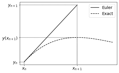
Another way to see the Euler method is as approximating the solution \(y(x)\) as a straight line over the interval \([x_n, x_n + h]\), passing through the point \((x_n, y_n)\) with a gradient of \(f(x_n, y_n)\) (the tangent of \(y\) at that point):

Worked Example
Consider the ODE:
with the given initial conditions: \(y = 1\) at \(x = 0\).
This has an analytic solution of:
which we can compare our numerical solutions to.
Let’s say we want to find the value of \(y\) at \(x = 1\) numerically (it’s \(e\)). We shall choose a step size of \(h = 0.05\) when integrating this out. What we need to do is recursively apply Euler steps until we have reached the desired \(x\):
import numpy as np

x, y = 0, 1 #initial conditions

h = 0.05 #step size

x_end = 1 #the value of x for which we want to know y

#The ODE function
def f(x,y):
    return - 2 * (x -1) * y

#Iterating through the Euler method until x >= x_end:
while x < x_end:
    y = y + h * f(x,y)
    x = x + h #Note, we don't want to update x before it's used in the line above

print('y at x = 1 approximated using Euler: ', y)
print('y at x = 1: ', np.e)
y at x = 1 approximated using Euler:  2.7617285451021716
y at x = 1:  2.718281828459045
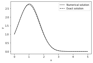
Now, it is often important for us to visualize the solution for \(y(x)\) over the interval, rather than only finding the value of \(y\) at the end of it. We will plot the numerical solution for \(y\) on the interval \(0 < x < 5\) along with the exact solution for comparison. We could alter the solution above to append the values to an array (as would be the best solution if we didn’t know how many iterations we needed), but instead we will create an array of \(x\) values on the interval, as this is known to us before perform the Euler solution:
import numpy as np
import matplotlib.pyplot as plt

x0, y0 = 0, 1
h = 0.05
x_end = 5

#The ODE function
def f(x,y):
    return -2 * (x - 1) * y

#Constructing the arrays:
x_arr = np.arange(x0, x_end + h, h) #make sure it goes up to and including x_end

y_arr = np.zeros(x_arr.shape)
y_arr[0] = y0

#Performing the Euler method, note we don't use the last x value in the update calculations
for i,x in enumerate(x_arr[:-1]):
    y_arr[i+1] = y_arr[i] + h*f(x, y_arr[i])

#Plotting the solution
fig, ax = plt.subplots()

ax.plot(x_arr, y_arr, color = '0.3', label = 'Numerical solution')
ax.plot(x_arr, np.exp( -(x_arr - 1)**2 + 1 ), 'k--', label = 'Exact solution')
ax.set_xlabel('x')
ax.set_ylabel('y')

ax.legend()

plt.show()

