.ipynb .pdf

repository open issue

Binder

Contents

Least Squares Minimization with scipy.optimize.leastsq

So far we have only considered functional relationships that are linear in the unknown constants. Non-linear cases are far more complicated and generally require numerical solutions. We will use a function from the SciPy module scipy.optimize, which contains functions for minimization, least squares and root finding techniques.

An Example of a Nonlinear Model

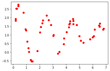
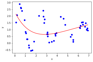
Consider the data found in the data file nonlinear_data.csv on GitHub , plotted below:

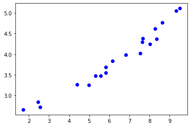
Though the data may appear to follow a linear trend, this is not the case. Consider the linear fit below:

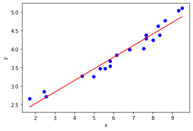
Instead a more appropriate functional relation is an exponential function:

\[ y = a_0 + a_1 e^{a_2 x} \]

Note that this functional relation is non-linear in \(a_2\). Applying the method of least squares minimization to this functional relation will not yield an analytic solution, therefore a numerical method is required. We shall not be implementing this numerical method ourselves, instead using a function from SciPy to solve our problem. In short the numerical minimization technique involves following the negative gradient (or an approximation of this) from a given starting point, until a local minimum is found (essentially the solution is captured here).

Nonlinear Least Squares Minimization with scipy.optimize.leastsq

The SciPy module scipy.optimize contains functions for minimization, least squares and root finding techniques. Of particular interest to us now is the leastsq function (documentation here), which we shall use to perform nonlinear least squares minimization.

The call signature of leastsq, including only the arguments of immediate interest to us, is:

leastsq(func, x0, args = () )

The x0 argument is an initial guess for the unknown parameters we are trying to find (required by the numerical minimization technique). In our case this is an initial guess for the \(a_j\) constants.

The keyword argument args is a tuple of the variables or data we are fitting the model to. In our case \(x\) and \(y\). The order in which these variables are presented is up to you, but must correspond to the order they are used in func. Each element of this tuple should be an array or list of data points, for instance (xdata, ydata).

The func argument is a callable object (function). It is referred to as the residual. It is the sum of the residuals squared that will be minimized.For the sum of errors squared the residual is equivalent to our error terms (\(\epsilon_i\)).

\[ S^2 = \sum_{i = 1}^{N} \text{func(arguments)}^2 \]

The call signature of func is:

func(params, *args)

where params is a list or array of the parameters we are trying to find (\(a_j\)), and args is the tuple of the data for our variables (\(x\) and \(y\)).

The * operator before a sequence data structure in a function argument unpacks that data structure as if each element where entered into the function individually. For example f( *(x,y,z) ) is equivalent to f(x, y, z)

The return value of the leastsq function (if it is only given the arguments listed above) is a tuple containing the solution for the \(a_j\) and an integer flag (for which a value between 1 and 4 indicates the solution was found).

Worked Example

Let’s use scipy.optimize.leastsq to fit the functional relation:

\[\begin{align*} y &= a_0 + a_1 e^{a_2 x}\\ &= f(x; \vec{a}) \end{align*}\]

to the nonlinear_data.csv.

Firstly we shall define the functional relation:

def f(a, x):
    return a[0] + a[1] * np.exp(a[2] * x)

and use this to define the residuals. For regular least-squares, we will use the error as the residuals:

\[ \epsilon = f(x; \vec{a}) - y \]

in Python this looks like:

def err(a, x, y):
    return f(a, x) - y

Putting this into action:

import numpy as np
import matplotlib.pyplot as plt

#importing scipy.optimize.leastsq only
from scipy.optimize import leastsq

#The model to fit to the data
def f(a, x):
    return a[0] + a[1] * np.exp(a[2] * x)

#Residuals (in this case the error term)
def err(a, x, y):
    return f(a, x) - y

#Reading the data
# The `unpack` keyword argument seperates the columns into individual arrays 
xdata, ydata = np.loadtxt('data/nonlinear_data.csv', delimiter = ',', unpack = True) 

#Performing the fit
a0 = [1.5, 0.6, 0.2] #initial guess

a, success = leastsq(err, a0, args = (xdata, ydata))

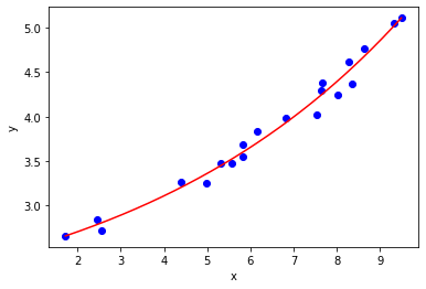
#Plotting the fit and data
x = np.linspace(xdata.min(), xdata.max(), 1000)

plt.plot(xdata, ydata, 'bo')
plt.plot(x, f(a, x), 'r-')
plt.xlabel('x')
plt.ylabel('y')
plt.show()

Solutions Converging on Local Minima

As mentioned before, the numerical algorithm is complete once it has minimized the objective function (the sum of errors squared in out case) to a local minimum. It is possible for the solution to not represent the global minimum, which is the ideal solution to obtain.

Let’s take a relatively simple example to illustrate this. Consider the functional relation:

\[ y = a_0 + a_1 e^{-a_2 x} \sin(a_3 x) \]

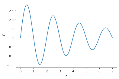
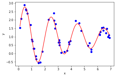
Given a set of data characterized by this relation:

It is relatively easy to find a good fit using leastsq:

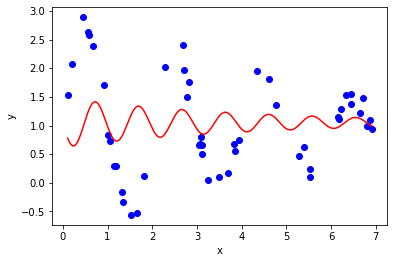
Here are a couple of examples of solutions that returns a supposedly successful solution, but have obviously not converged to the best fit.

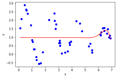
Here is an example of a solution that has not succeded (returned an integer flag greater than 4):

/home/mayhew/anaconda3/lib/python3.7/site-packages/scipy/optimize/minpack.py:449: RuntimeWarning: Number of calls to function has reached maxfev = 1000.
  warnings.warn(errors[info][0], RuntimeWarning)

If your model does not fit, try varying the initial guess for the fit parameters.

Multivariate Linear Least Squares Minimization Numerical Solutions to Ordinary Differential Equations