.ipynb .pdf

repository open issue

Binder

Contents

Simpson’s Rule

A way to interpret the trapezoidal method is that we approximate the integrand curve as a straight line, and then integrate that directly. The Simpson’s method does something similar, but instead of only using the integrand values at the boundaries it uses a third point (the midpoint) to approximate the integrand as a parabola.

The method approximates the integral as:

\[ \int_a^b f(x)~ dx \approx \frac{b - a}{6} \left[ f(a) + 4 f\left(\frac{a + b}{2}\right) + f(b)\right] \]

with the derivation of this in the following section.

Derivation

Approximating \(f(x)\) as a Quadratic Polynomial

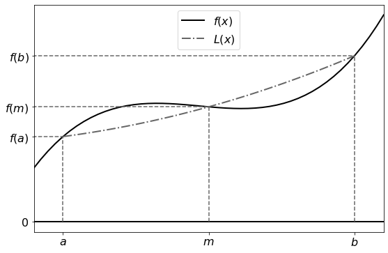
In order to approximate \(f(x)\) as a quadratic polynomial we can use a second order Lagrange polynomial. We construct this polynomial by using 3 data points \((a, f(a))\), \((m, f(m))\) and \((b, f(b))\).

\[ L(x) = f(a) \frac{(x - m)(x - b)}{(a - m)(a - b)} + f(m) \frac{(x - a)(x - b)}{(m - a)(m - b)} + f(b) \frac{(x - a)(x - m)}{(b - a)(b - m)} \]

If we use the midpoint of \([a, b]\) for \(m\), i.e:

\[ m = \tfrac{1}{2} (a + b) \]

then we have

\[ m - a = b - m = \tfrac{1}{2} (b - a) \]

and the Lagrange polynomial becomes:

\[ L(x) = \frac{2}{(b - a)^2} \big[ f(a) (x - m) (x - b) - 2 f(m) (x - a) (x - b) + f(b)(x - a)(x - m) \big] \]

Integrating \(L(x)\)

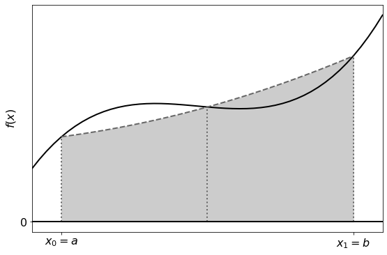
Now, we wish to approximate the integral of \(f(x)\) as the integral of our Lagrange polynomial:

\[ \int_a^b f(x)~ dx \approx \int_a^b L(x)~ dx \]

illustrated in the figure below:

by substituting the variable:

\[ u = \frac{x - m}{b - m} = 2 \frac{x - \tfrac{1}{2} (a + b)}{b - a} \]

into the integral of \(L(x)\) we find that:

\[ \int_a^b L(x)~dx = \frac{b - a}{6} \left[ f(a) + 4 f\left(\frac{a + b}{2}\right) + f(b) \right] \]

thus, we approximate the integral of \(f(x)\) as:

\[ \int_a^b f(x) ~dx \approx \frac{b -a}{6} \left[f(a) + 4 f\left(\frac{a + b}{2}\right) + f(b) \right] \]

Alternative Derivation

Another way to see the Simpson’s rule is as a weighted average of the midpoint and trapezoidal rules:

2/3 midpoint + 1/3 trapezoidal

Mathematically:

\[\begin{align*} \int_a^b f(x)~ dx &\approx \frac{2}{3} f\left(\frac{a + b}{2}\right) (b - a) + \frac{1}{3} \times \frac{1}{2} (b - a) [f(a) + f(b)]\\ &\approx \frac{b - a}{6} \left[ f(a) + 4 f\left(\frac{a + b}{2}\right) + f(b)\right]\\ \end{align*}\]

Composite Simpson’s Rule

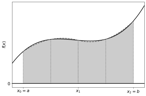
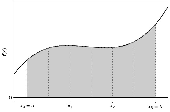
As before we can improve the accuracy of our solution by subdividing the interval and calculating the integral using Simpson’s rule for each subinterval.

The composite Simpson’s rule is given by:

\[\begin{split} \int_a^b f(x)~ dx \approx \sum_{i = 1}^n \frac{x_i - x_{i-1}}{6} \left[ f(x_{i-1}) + 4 f\left(\frac{x_{i-1} + x_i}{2}\right) + f(x_i)\right]\\ \end{split}\]

If we use equal sized subintervals, then we have that:

\[ x_i - x_{i -1} = \frac{b - a}{n} \]

taking this into account and the values of \(f(x_i)\) which are repeated in the sum, the composite Simpson’s rule can be simplified to:

\[ \int_a^b f(x)~ dx \approx \frac{b - a}{6 n} \left[ f(a) + 2 \sum_{i = 2}^{n-1} f(x_i) + 4 \sum_{i =1}^{n} f\left( \frac{x_{i-1} + x_i}{2} \right) + f(b) \right] \]

Assuming that \(0 < \tfrac{b - a}{6 n} < 1\), then the error for this method is \(O\left(\tfrac{1}{n}^4\right)\) [IntSimp1]

Composite Simpson’s Rule with a Discrete Data Set

Again, consider the data set \((x_i, y_i)\) for \(i = 0, \dots, n\), where

\[ f(x_i) = y_i \]

Approximating the integral of the data using Simpson’s rule is a lot less straight forward than the Midpoint and Trapezoidal rule as we can’t calculate \(f\left((x_{i -1} + x_i)/2\right)\) directly, and the function values at the boundaries of the intervals are also required.

If the \(x_i\) values are uniformly spaced (with \(x_i - x_{i-1} = \Delta x\)) and there is an odd number of data points, we can pair up the intervals between the points. Treating each pair of subintervals as a single subinterval, we can use the middle \(x\) values as the midpoints. In other words, for even \(i= 2j\), the \(x_{2j}\) are used as the boundaries of the sub-intervals; for odd \(i = 2k -1\), the \(x_{2k-1}\) are used as the midpoints of the subinterval. Thus the integral is approximated as:

\[ \int_{x_0}^{x_n} f(x)~dx \approx \frac{\Delta x}{3} \left[y_0 + 2 \sum_{i = 1}^{n/2 - 1} y_{2i} + 4 \sum_{i=1}^{n/2} y_{2i-1} + y_n \right] \]

Note that

\[ \frac{b - a}{6 n} = \frac{2 \Delta x}{6} = \frac{\Delta x}{3} \]

as each subinterval is made up of two intervals of length \(\Delta x\) each.

References

IntSimp1

James F. Epperson. An Introduction to Numerical Methods and Analysis. John Wiley & Sons, Inc., Hoboken, New Jersey, second edition edition, 2013.

Trapezoidal Rule